

This page tries to give some background information on how PlasmaMR
decomposes a job into tasks, and which task types are used. In this
respect PlasmaMR is very different from other map/reduce
implementations, as it employs fine-grained job
decomposition. This means that all processing steps reading or
writing files are considered as a task, and not only those steps that
drive the user-specified map and reduce functions. This approach
raises interesting questions about what the best decomposition is, as
we'll see.
As all data files reside in PlasmaFS (and there are no files in the local filesystem), every task can be principially run on every node. If the PlasmaFS files accessed by the task are stored on the same node, the accesses are very fast (even shared memory is used to speed this data path up). If the files are stored on a different node, PlasmaFS is responsible for making the files available via network. On the one hand this raises the transport costs, but on the other hand more CPU cores can be used (or more flexibly used) to execute the tasks. Of course, there are lots of ways of assigning tasks to nodes, and some are better than others. We discuss this in more detail below.
The input data
Before the job is decomposed, the input data is analyzed. The input data can be given as one or several PlasmaFS files, with or without block replication. The data is now cut into pieces, so that
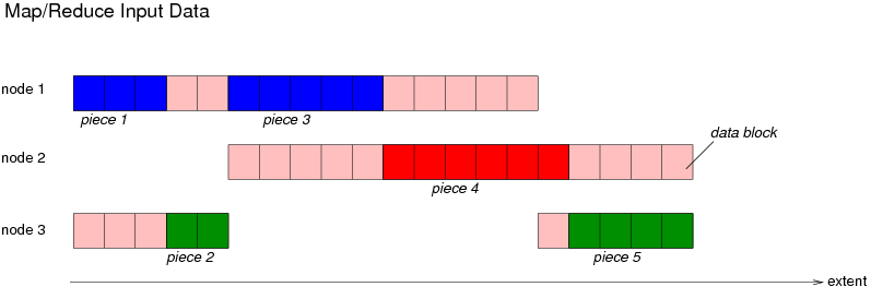
This picture show a file with a replication factor of two, i.e. each data block is stored on two nodes. The system splits the file up into five pieces (red, blue and green block ranges). Because each block is available on two nodes, it is possible to select each block from two nodes. It is now tried to make the block ranges as large as possible while creating enough pieces in total.
Formally, each piece is described as a list of block ranges coming
from input files (see types Mapred_tasks.file and
Mapred_tasks.file_fragment). In the following, we refer to this
input as "pieces of input data", and D be the number of pieces.
The task types
Right now, the following types are implemented:
map function to the input, and write the results to new intermediate
files. Each Map task creates at least one file but it will create more
than one if the amount of data exceeds the sort limit. As these intermediate
files are further processed by Sort tasks it is possible to apply an
optimization
here. Sorting is easier to do if it is known in advance how much data is
to be sorted. By keeping the size of the intermediate files below the
sort limit, the Sort tasks can be written so that all sorting occurs
in RAM.
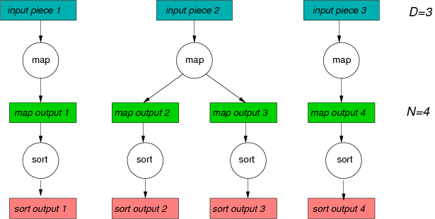
Here, we found three input pieces, and each piece is mapped to a
map output. For the second map operation we got more output than
sort_limit allows, and hence two map output files are created.
So the Map round of tasks created four output files in total, and
each of these files is sorted.
After sorting, the data is available in this form: There are N sorted files where each file stems from one input piece. There can be more sorted files than input pieces, i.e. N can be larger than D. The remaining algorithm needs now to merge all these sorted files, and it has to split the data into P partitions at the same time (remember that the keys of the records are partitioned into P sets). We call these sets "partition 0", ..., "partition P-1".
Merging and partitioning is done by applying the following type of task several times:
merge_limit and split_limit.s output files:
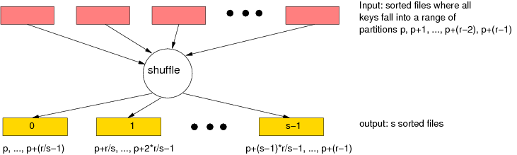
For the inputs we already know that the keys of the inputs fall into a
range of r partitions. The outputs are now further split in a way so
that each of the s files contains the records from partition ranges
that are s times smaller.
This task type allows a lot of constructions. For example, one could first merge all the N sort output files to a single file, and then split this file into P partitions, i.e. we first run Shuffle tasks where only merging happens, and then Shuffle tasks with only splitting. Another construction would do the converse: First split the N sort outputs further up into N*P smaller files, and then merge these files into P partitions. However, what PlasmaMR really does is a mixture of both approaches: In several rounds of data processing, Shuffle tasks are run that both merge and split to some extent. This is seen as best method because it allows a lot of parallel processing while not creating too many intermediate files. It is explained in more detail below.
is_reduce flag is set.
This enables that the user-defined reduce function is run.
Reduce tasks are only created in the final step of shuffling, i.e.
when the output files are the final output files of map/reduce.
Also, it is (for now) required that no splitting occurs.
map function on a piece of input data. The
result is split into several output sets (kept in RAM buffers).
Whenever the sets reach a size comparable to sort_limit, the
sets are sorted in RAM, and finally written to output files,
split by partition ranges.
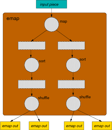
The scheduler only creates Emap tasks when it is configured to do
so. The number of output sets is a parameter
(Mapred_def.mapred_job_config.enhanced_mapping). Experimentation
showed so far that Emap is not always an improvement, in particular
because a higher number of intermediate files are created, resulting
in higher data fragmentation, and more work for merging data.
Constructing execution graphs
PlasmaMR represents execution graphs explicitly (in Mapred_sched):
The execution order of the tasks is not hard-coded in a fixed
algorithm, but the order of steps is expressed as a graph where
vertexes represent either data or tasks, and the edges represent the
data flow (and implicitly the execution order). This has a number
of advantages:
-simulate of the exec_job command) - easing research on
graph constructionexec_job)As a better alternative, the graph is extended so far possible whenever an executed Map or Emap task has produced outputs. This means that dependent tasks are added as soon as possible, and generally more tasks are considered as executable in the construction/execution process.
Another advantage of the iterative construction is that even the locality of files (i.e. on which nodes files are really stored) can sometimes be used to optimize the graph.
Execution graphs with Map, Sort, and Shuffle
The following diagam shows an execution graph for D=N=3 and for P=4 partitions:
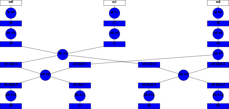
Notation:
M: Map tasksSO: Sort tasksSH: Shuffle tasks#n: the task ID (assigned at execution time)mn: input piece to map number nsn: map or sort output number nsm-n/pu-v: this file contains data from
sm to sn falling into the partitions u to vpu: output partition ureduce function).
The graph can be analyzed in the following ways:
-dump-svg
switch of exec_job. When generating diagrams for larger jobs, the
following observations are easier to make.
Roughly, the graph is executed top to bottom. The possible
parallelism is limited by the number of tasks in the same row. For
instance, this diagram has a row with only SH #6 and SH #7, so at
this point of execution only these two tasks can run at the same time.
Another observation is that the locality of the data increases from
top to bottom. For example, once SH #6 and SH #7 are done, the
whole data set is split into two independent halves. If each half was
executed on its own machine, there was no need for a task on one
machine to get the output of a task that ran on the other machine.
Generally, once the number of partitions exceeds the number of nodes,
there is no need anymore to access data over the network.
In each round of data processing (as indicated by the "rows" of the diagram) a certain number of files is merged, and the data is again split into a certain number of files. If now D and P are roughly in the same order of magnitude, the sizes of the files will not dramatically change from round to round. Especially, very small files are avoided, and random disk seeks are never required to gather up small fragments from the disk.
Execution graphs with Emap and Shuffle
Assigning tasks to nodes
